Julia is a relatively young technical computing language. One of its features is JuMP (Julia for Mathematical Programming), a powerful package that allows mathematical models to be built and solved within the Julia environment. My first blog post offered a simple model for scheduling the Big Ten conference in a round-robin tournament. To complete the Circle of Life, this final blog post will revisit the model by implementing it in Julia/JuMP.
First things first! Let’s tell Julia we need to use the JuMP package for creating a model and the CPLEX package for accessing the CPLEX solver.
using JuMP, CPLEX
Previously, we defined a set 


M = ["Ind" "UMD" "UMich" "MSU" "OSU" "Penn" "Rtgrs" "Ill" "Iowa" "UMN" "UNL" "NU" "Purd" "UW"]
D = collect(1:13)
We now create a JuMP model object with CPLEX as the solver. This model will have variables, constraints, and an objective added to it. CPLEX options can be passed as arguments into the CplexSolver object; e.g., CPX_PARAM_THREADS=4.
model = Model(solver=CplexSolver())
The binary decision variables will be 


@variable macro. JuMP is even kind enough to allow us to index our variables with our team names!
@variable(model, x[M,M,D], Bin)
Obviously, a team can’t play itself. Let’s set all binary variables of the form 
@constraint macro.
for i in M
	for t in D
		@constraint(model, x[i,i,t] == 0)
	end
end
Our original model included the constraint that each team can play at most once per day, whether they are home or away. The mathematical formulation of this constraint is below.

The following code in Julia adds this exact constraint to our model. We add this constraint for every combination of teams (
for i in M
	for t in D
		@constraint(model, sum{x[i,j,t] + x[j,i,t], j in setdiff(M,[i])} <= 1)
	end
end
The sum function sums the expression 

setdiff(M,[i]).
Because we want a round-robin schedule, each team must play every other team exactly once. In the first blog post, we saved ourselves from adding redundant constraints by adding a constraint for all 


We add this constraint to the JuMP model for all
for i in 1:length(M)
	for j in M[i+1:end]
		@constraint(model, sum{(x[M[i],j,t] + x[j,M[i],t]), t in D} == 1)
	end
end
So far, there’s nothing in our model that prevents a team from playing all home or all away games. Let’s make sure each team plays either 


In Julia, we will implement this constraint by simultaneously summing over the two indices mentioned above: 
for i in M
	@constraint(model, sum{x[i,j,t], j in setdiff(M,[i]), t in D} >= ceil((length(D) - 1)/2))
end
The final constraints explicitly provided in the first blog post limited the number of consecutive home and away games. This is important to facilitate a healthy, “mixed” schedule. These constraints stated that a team cannot play more than two home games within any consecutive three-game window. Similarly, teams cannot play more than two away games within any consecutive three-game window.


The JuMP analog of these constraints again sums over two indices simultaneously.
for i in M
	for t in 1:length(D)-2
		@constraint(model, sum{x[i,j,s], j in M, s in t:t+2} >= 2)
		@constraint(model, sum{x[j,i,s], j in M, s in t:t+2} >= 2)
	end
end
These are all of the constraints we added to the original model. All that’s left is to solve the model.
status = solve(model)
The solve command will return a symbol, stored in the status variable, that lets us know how the model solved. It could take on a value of :Optimal, :Unbounded, or :Infeasible, among other values. Fortunately for us, this model returned an “optimal” value. Remember that at this point, we are just searching for a schedule feasible for our constraints. After tidying up the output, we have a complete schedule.

However, this may not be the perfect schedule. Notice that there are 23 instances of teams playing back-to-back away games. Let’s say we wanted to reduce this number as much as possible. How would we do it?
One way to minimize the total number of back-to-back away games is to introduce a binary variable 

@variable(model, y[M,1:length(D)-1], Bin)
These variables should be triggered to equal
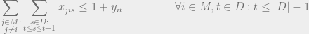
The JuMP constraint looks very similar to the previous “window” constraints.
for i in M
	for t in 1:length(D)-1
		@constraint(model, sum{x[j,i,s], j in M, s in t:t+1} <= 1 + y[i,t])
	end
end
The last step is to add an objective function to our JuMP model. We want to minimize the total number of

Objective functions are added to JuMP models with the @objective macro. We declare the sense of the objective function to be Min because we are minimizing our linear objective. Summations in the objective function behave the same way as they do in the constraints.
@objective(model, Min, sum{y[i,t], i in M, t in 1:length(D)-1})
Our model is complete! After executing the solve(model) command once more, we have a new solution. This new model is very difficult to solve, so we present an improved solution obtained after running the solver for a few minutes.

This schedule features 7 instances of back-to-back away games. This is an enormous improvement to our earlier solution!
JuMP is also capable of more advanced solving techniques, such as solver callbacks for lazy constraints and user cuts. If you’re interested in trying out Julia/JuMP, you can download Julia here. Packages are incredibly easy to add to your Julia distribution (Pkg.add("JuMP")). Happy optimizing!

Thank you for this gentle introduction to optimization in Julia and for circling back to your first post.
LikeLike
Felix the Cat Rules!
LikeLike